Research on Non-linear Phenomena in Ship Motion
Index
In our laboratory, we are conducting a number of studies on nonlinear phenomena.
Fractals in Capsizing of a Ship in Regular Waves
The movement of a ship is non-linear, and strange results can be obtained from really simple equations that you might learn in a second year undergraduate class. The video below shows the result of solving the equation of motion of the ship and determining capsizing and non-capsizing, but a mysterious pattern appears. This is known as fractal.
The banana-like erosion shape shown in this video, to put it a little harder, matches the shape of the stable manifold at the left and right saddle-shaped unstable equilibrium points. The fractals represents complicated phenomenon sunch as bifurcation, chaos, symmetry breaking, etc., but it is interesting to note that the complicated patterns can be generated using a very simple equation of forced ship roll motion as shown below.
A set of sample codes to generate the fractals is provided below,
Python Code
#   Visualization of Fractal in Capsizing Equation
#
#   Coded by Atsuo MAKI, Ryohei SAWADA and Kouki WAKITA (JFY-R3/4/25)
#   Ship Intelligentization Subarea, Osaka University
#
#   The equation and parameter set are based on the paper of Dr.Kan as follows
#   Kan, M. and Taguchi, H., Capsizing of a Ship in Quatering Seas,
#   Journal of the Society of Naval Architects of Japan, vol.168, pp.211-220, 1990
#   https://doi.org/10.2534/jjasnaoe1968.1990.168_211
#
import math

import numpy as np
import matplotlib.pyplot as plt
from scipy.integrate import odeint, solve_ivp


class Config:
	"""Config

	NDIV: number of time discretization
	OMEGA: frequency of external wave moment
	KAPPA: damping coefficient
	B: Amplitude of external moment
	PDIV: In order to show time history, set conf.pdiv = 1.
				If not, set 2 or over. Use large value such as conf.pdiv = 100.
	ROLL_MAX: absolute value of maximum value of roll angle in search domain
	RATE_MAX: absolute value of maximum value of roll angular rate in search domain
	T: natural roll period
	DT: dicritized time in numerical simulation defined as T / NDIV
	MAXT: final time in numerical simulation
	"""

	NDIV = 100
	OMEGA = 0.905
	KAPPA = 0.04455
	B = 0.12
	PDIV = 100
	ROLL_MAX = 1.5
	RATE_MAX = 1.5
	BY_SCIPY = True
	FIG_DIR = "./figure.png"

	def __init__(self):
		self.T = 2.0 * math.pi / self.OMEGA
		self.DT = self.T / self.NDIV
		self.MAXT = 100 * self.T


def set_config():
	return Config()


def right_cal(t, y, conf):
	"""Definition of right side of the differential equation

	Args:
		t (numpy.float64): time (s)
		y (numpy.ndarray): y[0]:roll angle, y[1]:roll angler rate
		conf (Config): parameter

	Returns:
		right: right hand side of state equation
	"""
	right = np.array([
		y[1],
		- conf.KAPPA * y[1] - y[0] + y[0]**3 +
		conf.B * math.cos(conf.OMEGA * t)
	])
	return right


class RollCapsizing:
	"""Class contains functions to be used
	"""

	def __init__(self, conf):
		self.conf = conf

	@staticmethod
	def get_capsize_detection():
		"""Capsizing detection used in solve_ivp func.
		"""
		def capsize_detection(t, x):
			return abs(x[0]) - math.pi
		capsize_detection.terminal = True
		capsize_detection.direction = 0
		return capsize_detection

	def calc_time_history(self):
		"""Calculate time history of roll motion

		Returns:
			sol.t: time
			sol.y[0]: roll angle
			sol.t_events[0]: time to capsize
		"""
		sol = solve_ivp(
			lambda t, y: right_cal(t, y, self.conf),
			t_span=(0, self.conf.MAXT),
			y0=np.array([-self.conf.RATE_MAX, -self.conf.ROLL_MAX]),
			method='RK45',
			max_step=self.conf.DT,
			# min_step=self.conf.DT,
			events=self.get_capsize_detection())
		return sol.t, sol.y[0], sol.t_events[0]

	def judge_cap_in_grid(self):
		"""Numerical calculation and judge capsizing for each parameter

		Returns:
			cap_roll: initial roll angle which leads to capsizing
			cap_rate: initial roll angular rate which leads to capsizing
		"""
		cap_roll = []
		cap_rate = []
		int_rate_list = np.linspace(
			-self.conf.RATE_MAX, self.conf.RATE_MAX, self.conf.PDIV+1)
		int_roll_list = np.linspace(
			-self.conf.ROLL_MAX, self.conf.ROLL_MAX, self.conf.PDIV+1)
		for i_rate, int_rate in enumerate(int_roll_list):
			for i_roll, int_roll in enumerate(int_roll_list):
				if self.conf.BY_SCIPY:
					cap_occur = self.judge_cap_by_scipy(
						int_rate, int_roll)
				else:
					cap_occur = self.judge_cap_by_myrk4(
						int_rate, int_roll)
				print(f"rate {i_rate} / {self.conf.PDIV}: roll: {i_roll} / {self.conf.PDIV}", end='\r')
				if cap_occur == False:
					cap_roll.append(int_roll)
					cap_rate.append(int_rate)
		return cap_roll, cap_rate

	def judge_cap_by_scipy(self, int_rate, int_roll):
		"""numerical calculation and judge capsizing (this function uses solve_ivp in scipy)

		Args:
			int_rate (numpy.float64): initial roll angular rate
			int_roll (numpy.float64): initial roll angle

		Returns:
			bool: True = capsizing, False = not-capsizing
		"""
		sol = solve_ivp(
			lambda t, y: right_cal(t, y, self.conf),
			t_span=(0, self.conf.MAXT),
			y0=np.array([int_roll, int_rate]),
			method='RK45',
			t_eval=(0, self.conf.MAXT),
			events=self.get_capsize_detection()
		)
		return len(sol.t_events[0]) != 0

	def judge_cap_by_myrk4(self, int_rate, int_roll):
		"""numerical calculation and judge capsizing (this function uses my 4th order Runge-Kutta)

		Args:
			int_rate (numpy.float64): initial roll angular rate
			int_roll (numpy.float64): initial roll angle

		Returns:
			bool: True = capsizing, False = not-capsizing
		"""
		def f(t, y): return right_cal(t, y, self.conf)
		y = np.array([int_roll, int_rate])
		t_series = np.arange(
			0, self.conf.maxT + self.conf.DT, self.conf.DT
		)
		cap_d = self.get_capsize_detection()
		for t in t_series:
			k_1 = f(t, y)
			k_2 = f(t + self.conf.DT / 2.0, y + self.conf.DT * k_1 / 2.0)
			k_3 = f(t + self.conf.DT / 2.0, y + self.conf.DT * k_2 / 2.0)
			k_4 = f(t + self.conf.DT, y + self.conf.DT * k_3)
			y += self.conf.DT * (k_1 + 2 * k_2 + 2 * k_3 + k_4) / 6
			if cap_d(t, y) > 0:
				return True
		return False


def calc_roll_cap(conf):
	rc = RollCapsizing(conf)
	return rc.judge_cap_in_grid()


def calc_roll_history(conf):
	rc = RollCapsizing(conf)
	return rc.calc_time_history()


def draw_figure(cap_roll, cap_rate, conf):
	"""Draw fractal plot in case of conf.PDIV > 1

	Args:
		cap_roll (list): initial roll angle which leads to capsizing
		cap_rate (list): roll angular rate which leads to capsizing
		conf (Config): config
	"""
	# font
	plt.rcParams['font.size'] = 12
	plt.rcParams['font.family'] = 'Times New Roman'
	# make tick direction inside
	plt.rcParams['xtick.direction'] = 'in'
	plt.rcParams['ytick.direction'] = 'in'
	# set color
	gainsboro = [220 / 255, 220 / 255, 220 / 255]
	# set axis
	fig = plt.figure(figsize=(8.0, 8.0), facecolor='w')
	ax = fig.add_subplot(1, 1, 1)
	ax.set_xlim([-1.5, 1.5])
	ax.set_ylim([-1.5, 1.5])
	# x-y axis
	ax.yaxis.set_ticks_position('both')
	ax.xaxis.set_ticks_position('both')
	# set labels
	fig.suptitle(
		'White region is the initial condition which leads to capsizing.')
	ax.set_xlabel('roll [ rad ]')
	ax.set_ylabel('roll rate [ rad / sec ]')
	# Text box
	str_annotation = ' B = ' + str(conf.B)
	text_dict = dict(boxstyle="round4",
						facecolor=gainsboro, edgecolor="black")
	# show annotation (box style)
	ax.annotate(
		str_annotation,
		xy=(-1.25, 1.25),
		bbox=text_dict,
		size=15, color="black")
	# plot
	ax.scatter(cap_roll, cap_rate, s=5, c='black', edgecolors=None)
	# save
	fig.savefig(conf.FIG_DIR)


def draw_time_series(t, y, t_cap_occur, conf):
	"""Draw time series in the case of conf.PDIV == 1

	Args:
		t (numpy.ndarray): time
		y (numpy.ndarray): soltuion of differential equation in time domain
		t_cap_occur (numpy.ndarray): time to capsize
		conf (Condig): config
	"""
	# font
	plt.rcParams['font.size'] = 12
	plt.rcParams['font.family'] = 'Times New Roman'
	# make tick direction inside
	plt.rcParams['xtick.direction'] = 'in'
	plt.rcParams['ytick.direction'] = 'in'
	plt.rcParams['mathtext.fontset'] = 'stix'
	#   set color
	crimson = [220 / 255, 20 / 255, 60 / 255]
	#   set axis
	fig = plt.figure(figsize=(8.0, 8.0/1.67), facecolor='w')
	ax = fig.add_subplot(1, 1, 1)

	if len(t_cap_occur) == 0:
		ax.set_xlim([0, conf.maxT])
	else:
		ax.set_xlim([0, t_cap_occur])
	ax.set_ylim([-math.pi, math.pi])
	# x-y axis
	ax.yaxis.set_ticks_position('both')
	ax.xaxis.set_ticks_position('both')
	# set title and label
	if len(t_cap_occur) == 0:
		str_title = 'time series (not capsizing)'
	else:
		str_title = 'time series (capsizing)'
	fig.suptitle(str_title)
	ax.set_xlabel('time [ s ]')
	ax.set_ylabel('roll [ rad ]')
	# plot
	ax.plot(t, y, color=crimson)
	# save
	fig.savefig(conf.FIG_DIR)


def main():
	conf = set_config()
	is_run_profiling = False
	if is_run_profiling:
		try:
			from line_profiler import LineProfiler
			print("Running profiling: calc_roll_cap \n")
			prof = LineProfiler()
			prof.add_function(calc_roll_cap(conf))
			prof.runcall(calc_roll_cap(conf))
			prof.print_stats()
		except ImportError:
			print('ImportError: line_profiler is not installed. If you want to profile the code, use pip and install it.')
			pass
	else:
		if conf.PDIV == 1:
			t, y, t_cap_occur = calc_roll_history(conf)
			draw_time_series(t, y, t_cap_occur, conf)
		else:
			cap_roll, cap_rate = calc_roll_cap(conf)
			draw_figure(cap_roll, cap_rate, conf)


#   Main program goes here
if __name__ == "__main__":
	main()
Julia Code
#
#   Fractal in Capsizing Equation
#   Coded by Ryohei SAWADA, Atsuo MAKI and Kouki WAKITA (JFY-R3/4/24)
#   The equation and parameter set are based on the paper of Dr.Kan as follows
#   Kan, M. and Taguchi, H., Capsizing of a Ship in Quatering Seas,
#   Journal of the Society of Naval Architects of Japan, vol.168, pp.211-220, 1990
#   https://doi.org/10.2534/jjasnaoe1968.1990.168_211
#

using PyPlot

# Calculation config.
Base.@kwdef struct Config
	ndiv::Int = 100
	ω::Float64 = 0.905 # frequency of external wave moment
	κ::Float64 = 0.04455 # damping coefficient
	t::Float64 = 2π / ω # natural roll period
	dt::Float64 = t / ndiv # time step of integration
	maxn::Int = 100 * ndiv
	b::Float64 = 0.12
	# In order to show time history, set config.pdiv = 1.
	# If not, set 2 or over. Use a large value such as config.pdiv = 100.
	pdiv::Int = 100
	roll_max::Float64 = 1.5
	rate_max::Float64 = 1.5
	droll::Float64 = roll_max * 2.0 / pdiv
	drate::Float64 = rate_max * 2.0 / pdiv
end

"""
	equation(t, y, config::Config)

Roll motion for capsizing simulation.
The first argument `t` is a time to calculate external force by wave.
The second argument `y` is a vector of the roll angle and the rate of rolling.
The configration of equation is given as a `Config` struct.
"""
function equation(t, y, config::Config)
	return [y[2], - config.κ * y[2] - y[1] + y[1]^3 + config.b * cos(config.ω * t)]
end

"""
	calc_roll_capsize(config::Config=Config())

Capsizing simulation.
Integration is done by RK4.
"""
function calc_roll_capsize(config::Config=Config())
	# Initialization
	iscap = zeros(Bool, config.pdiv, config.pdiv) # flg mat. for capsizing or not.
	cap_roll = Float64[] # capsizing simulation result of roll
	cap_rate = Float64[] # capsizing simulation result of rolling rate
	for i_rate in 1:config.pdiv
		ini_rate = - config.rate_max + i_rate * config.drate
		for i_roll in 1:config.pdiv
			flush(stdout)
			print(" rate: $(lpad(string(i_rate), 3, "0")) / $(config.pdiv) roll: $(lpad(string(i_roll), 3, "0")) / $(config.pdiv) \r")
			t = 0.0
			ini_roll = - config.roll_max + i_roll * config.droll
			y0 = [ini_roll, ini_rate]
			y = y0[:] # deepcopy
			iscap[i_roll, i_rate] = false
			# Integration with Runge-Kutta
			for i in 1:config.maxn
				k_1 = equation(t, y, config)
				k_2 = equation(t + config.dt / 2.0, y + config.dt * k_1 / 2.0, config)
				k_3 = equation(t + config.dt / 2.0, y + config.dt * k_2 / 2.0, config)
				k_4 = equation(t + config.dt, y + config.dt * k_3, config)
				y += config.dt * (k_1 + 2.0 * k_2 + 2.0 * k_3 + k_4) / 6.0
				t += config.dt
				if abs(y[1]) > π # if capsizing
					iscap[i_roll, i_rate] = true
					break
				end
			end
			if iscap[i_roll, i_rate] == false
				append!(cap_roll, [y0[1]])
				append!(cap_rate, [y0[2]])
			end
		end
	end
	return cap_roll, cap_rate, config
end

"""
	draw_figure(cap_roll, cap_rate, config::Config=Config())

Draw figure from a simulation result by `calc_roll_capsize()`.
"""
function draw_figure(cap_roll, cap_rate, config::Config=Config())
	# set color
	gainsboro = [220 / 255, 220 / 255, 220 / 255]
	# set axis
	fig = PyPlot.figure(figsize=(8.0, 8.0), facecolor="w")
	PyPlot.xlim(- 1.5, 1.5)
	PyPlot.ylim(- 1.5, 1.5)
	PyPlot.PyDict(PyPlot.matplotlib."rcParams")["font.size"] = 12
	PyPlot.PyDict(PyPlot.matplotlib."rcParams")["font.family"] = "Times New Roman"
	# make tick direction inside
	PyPlot.PyDict(PyPlot.matplotlib."rcParams")["xtick.direction"] = "in"
	PyPlot.PyDict(PyPlot.matplotlib."rcParams")["ytick.direction"] = "in"
	# x-y axis
	PyPlot.gca().xaxis.set_ticks_position("both")
	PyPlot.gca().yaxis.set_ticks_position("both")
	# set labels
	fig.suptitle(
		"White region  is the initial condition which leads to capsizing.")
	PyPlot.xlabel("roll [ rad ]")
	PyPlot.ylabel("roll rate [ rad / sec ]")
	# Text box
	str_annotation = " B = $(config.b)"

	text_dict = Dict("boxstyle" => "round4", "facecolor" => gainsboro, "edgecolor" => "black")
	# show annotation (box style)
	PyPlot.gca().annotate(str_annotation,
						xy=(-1.25, 1.25),
						bbox=text_dict,
						size=15, color="black")
	#   plot
	PyPlot.scatter(cap_roll, cap_rate, s=5, c="black", edgecolors="None")
	#   draw now
	PyPlot.show()
end

function main()
	cap_roll, cap_rate, config = @time calc_roll_capsize()
	draw_figure(cap_roll, cap_rate)
end


if abspath(PROGRAM_FILE) == @__FILE__
	main()
end
The moment when a banana-like shape begins to appear can be estimated by a theoretical calculation method devised by a researcher named Melnikov as shown below.
When, \(\kappa=0.04455\) and \(\omega=0.905\), \(B\,(=B_{M})=0.0383\). In the above video there is a counter of \(B\), if you stop the video near this value, you can see that it is close to the condition where the banana shape starts to appear. The theory is quite interesting.
For example, the Saddle-Node bifurcation, which was one periodic solution for a small wave, is divided into three periodic solutions as the wave increases, and then the stable solution and the unstable solution annihilate, which can be easily observed from this equation.
Capsizing in Irregular Waves
But the actual waves are irregular. Then, can we use the approach and way of thinking about regular waves? The answer is yes. Recent research has made it possible to predict the probabilistic behavior of ship movements.What we use here is a stochastic process, especially a stochastic differential equation, which you may not learn in the undergraduate school. The one-dimensional stochastic differential equation for a certain quantity \(\mathcal{H}\) in the motion of a ship is given by,
The above equation is called Ito's stochastic differential equation. The steady-state FPK (Fokker-Planck-Kolmogorov) equation that corresponds to this equation is shown below.
\(\mathcal{P}(\mathcal{H})\) represents the probability density function which can be found from the equation below using the constant \(C\),
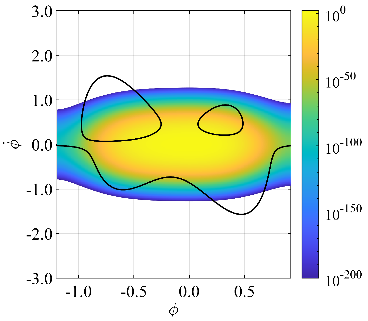
The probability density function of the ship's motion obtained by solving the problem in the irregular wave is shown below. The left is a numerical calculation and the right is a theoretical calculation. It's a good match. Don't you think the theory is amazing?
Such an approach allows the probabilistic calculation of ship capsizing. Furthermore, by applying this result, we are thinking about acceleration and its jerk of differential value using a new calculation method called PLIM (PDF Line Integral Method). The figure below shows the integration path of the line integral used at that time. It has a strange shape.